Generation of designs

The Orthogonal Array package can be used to generate several classes of arrays and designs. A collection of arrays and designs generated by the package is available on the website http://www.pietereendebak.nl/oapackage/index.html.

Generation of orthogonal arrays

A list of arrays in LMC form (i.e., lexicographically minimum in columns) can be extended to a list of arrays in LMC form with one additional column. Details about the algorithm are described in [SEN10].

The main function for array extension is the function extend_arraylist(). The arguments for this function are the list of arrays to extend, a specification of the class of arrays in arraydata_t and the options OAextend for the algorithm.

An example of a session that extends an array is:

>>> import oapackage
>>> nrows=8; ncols=3;
>>> arrayclass=oapackage.arraydata_t(2, nrows, 2, ncols)
>>> root_array=arrayclass.create_root()
>>> root_array.showarraycompact()
00
00
01
01
10
10
11
11
>>> array_list=oapackage.extend_array(root_array, arrayclass)
>>> print('found %d extensions of the root array' % len(array_list))
found 2 extensions of the root array

A more detailed example is included in Enumerate orthogonal arrays.

Conference designs

A conference design is an \(N\times k\) matrix with entries 0, -1, +1 such that i) in each column the symbol 0 occurs exactly one time and ii) all columns are orthogonal to each other. For details on conference designs, see the section Properties of conference designs and [SEG19]. An example of a session to generate conference designs is the following:

Generate conference designs with 8 rows

>>> import oapackage
>>> conference_class=oapackage.conference_t(8, 6, 0)
>>> array = conference_class.create_root_three_columns()
>>> array.showarray()
array:
  0   1   1
  1   0  -1
  1   1   0
  1   1   1
  1   1  -1
  1  -1   1
  1  -1   1
  1  -1  -1
>>> l4=oapackage.extend_conference ([array], conference_class, verbose=0)
>>> l5=oapackage.extend_conference ( l4, conference_class, verbose=0)
>>> l6=oapackage.extend_conference ( l5, conference_class, verbose=0)
>>> print('number of non-isomorphic conference designs with 6 columns: %d' % len(l6) )
number of non-isomorphic conference designs with 6 columns: 11

An example notebook with more functionality is included in Generation and analysis of conference designs. The full interface for conference designs is available in the Interface for conference designs.

The main functions to extend conference and double conference designs are extend_conference() and extend_double_conference(), respectively. The low-level functions for generating candidate extension columns of conference and double conference designs are generateConferenceExtensions() and generateDoubleConferenceExtensions(), respectively.

The conference designs are generated in LMC0 form.

Calculation of D-efficient designs

D-efficient designs (sometimes called D-optimal designs) can be calculated with the function oapackage.Doptim.Doptimize(). This function uses a coordinate-exchange algorithm to generate designs with good properties for the \(D\)-efficiency. With the coordinate-exchange algorithm, the following target function \(T\) is optimized:

\[T = \alpha_1 D_{\text{eff}} + \alpha_2 D_{s, \text{eff}} + \alpha_3 D_{1, \text{eff}}\]

Here, \(\alpha\) is a weight vector specified by the user. Details on the \(D_{\text{eff}}\), \(D_{s, \text{eff}}\) and \(D_{1, \text{eff}}\) can be found in the section Optimality criteria for D-efficient designs.

A Python script to generate D-efficient designs with 40 runs and 7 factors is shown below.

Example of Doptimize usage

>>> N=40; s=2; k=7;
>>> arrayclass=oapackage.arraydata_t(s, N, 0, k)
>>> print('We generate optimal designs with: %s' % arrayclass)
We generate optimal designs with: arrayclass: N 40, k 7, strength 0, s {2,2,2,2,2,2,2}, order 0
>>> alpha=[1,2,0]
>>> scores, dds, designs, ngenerated = oapackage.Doptimize(arrayclass, nrestarts=40, optimfunc=alpha, selectpareto=True, verbose=0)
Doptimize: iteration 0/40
Doptimize: iteration 39/40
>>> print('Generated %d designs, the best D-efficiency is %.4f' % (len(designs), dds[:,0].max() ))
Generated 10 designs, the best D-efficiency is 0.9198

The parameters of the Doptimize() function are documented in the code.

To calculate the \(D\)-, \(D_s\)- and \(D_1\)-efficiencies of the designs, we can use the method Defficiencies(). For details on these efficiencies, see the section Optimality criteria for D-efficient designs and [ES17].

In [ES17], it is shown that one can optimize a linear combination of the \(D\)-efficiency and \(D_s\)-efficiency to generate a rich set of good compromise designs. From the generated designs, the optimal ones according to Pareto optimality can be selected.

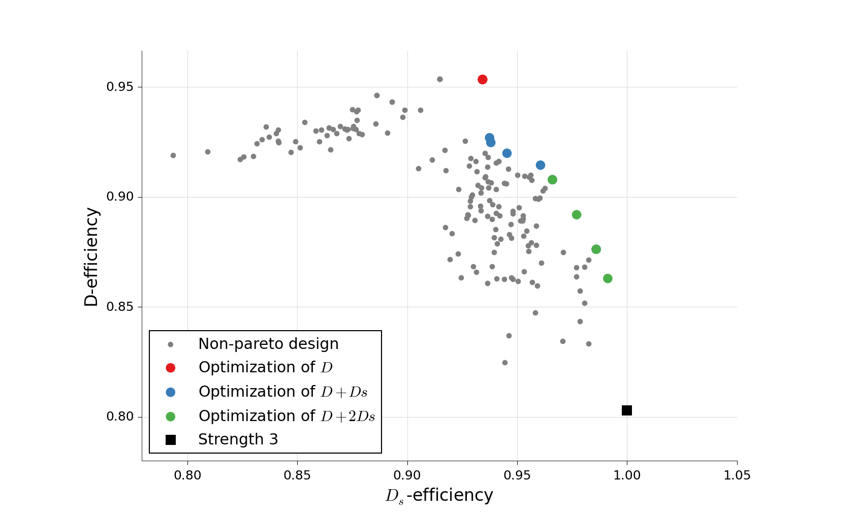
Scatterplot for the \(D\)-efficiency and \(D_s\)-efficiency for generated designs in \({\operatorname{OA}(40; 2; 2^7)}\). The Pareto optimal designs are colored, while the non-Pareto optimal designs are grey. For reference the strength-3 orthogonal array with highest D-efficiency is also included in the plot.

Even-odd arrays

The even-odd arrays are a special class of orthognal arrays with at least one of the odd \(J_k\)-characteristics unequal to zero. More information on this class of designs will appear later.